Initiation à la robotique Définition du problème
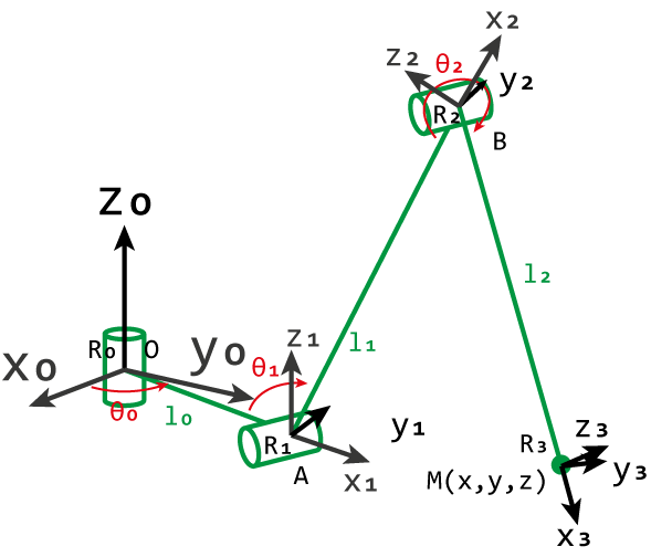
On cherche à trouver le modèle direct ie l'expression de ( x , y , z ) (x,y,z) ( x , y , z ) ( θ 0 , θ 1 , θ 2 ) (\theta_0, \theta_1, \theta_2) ( θ 0 , θ 1 , θ 2 ) ( θ 0 , θ 1 , θ 2 ) (\theta_0, \theta_1,
\theta_2) ( θ 0 , θ 1 , θ 2 ) ( x , y , z ) (x,y,z) ( x , y , z ) R \mathcal{R} R
Rappel sur la matrice de rotation
En 2D autour de 0 : r o t ( 0 , θ ) = ( cos θ − sin θ sin θ cos θ ) rot_{(0,\theta)} = \begin{pmatrix} \cos{\theta} & - \sin{\theta} \\\\
\sin{\theta} & \cos{\theta} \end{pmatrix} r o t ( 0 , θ ) = cos θ sin θ − sin θ cos θ
En 3D autour de 0 : r o t ( 0 , ( O , z ) , θ ) = ( cos ( θ ) − sin ( θ ) 0 sin ( θ ) cos ( θ ) 0 0 0 1 ) rot_{(0, (O,z), \theta)} =
\begin{pmatrix}
\cos(\theta) & -\sin(\theta) & 0 \\\\
\sin(\theta) & \cos(\theta) & 0 \\\\
0 & 0 & 1 \\\\
\end{pmatrix} r o t ( 0 , ( O , z ) , θ ) = cos ( θ ) sin ( θ ) 0 − sin ( θ ) cos ( θ ) 0 0 0 1
Modèle Direct
Soit la matrice A A A A = ( l 0 × cos θ 0 l 0 × sin θ 0 0 ) R A = \begin{pmatrix}
l_0 \times \cos{\theta_0} \\\\ l_0 \times \sin{\theta_0} \\\\ 0 & \end{pmatrix}_\mathcal{R} A = l 0 × cos θ 0 l 0 × sin θ 0 0 R
Soit la matrice B B B B = ( l 1 cos ( π − θ 1 ) 0 l 1 sin ( π − θ 1 ) ) R 1 B = \begin{pmatrix}
l_1 \cos{(\pi - \theta_1 )} \\\\ 0 \\\\ l_1 \sin{(\pi - \theta_1)}\end{pmatrix}_{\mathcal{R}_1} B = l 1 cos ( π − θ 1 ) 0 l 1 sin ( π − θ 1 ) R 1
r o t θ 0 , O z ⋅ B R 1 + A 2 ( cos θ − sin θ 0 sin θ cos θ 0 0 1 ) ⋅ ( l 1 cos ( π − θ 1 ) 0 l 1 sin ( π − θ 1 ) ) + ( l 0 cos θ 0 l 0 sin θ 0 0 ) \begin{align*}
rot_{\theta_0, \mathcal{O}_z} &\cdot B_{\mathcal{R}_1} + A_2 \\\\
\begin{pmatrix} \cos{\theta} & -\sin{\theta} & 0 \\\\
\sin{\theta} & \cos{\theta} \\\\
0 & 0 & 1 \end{pmatrix} &\cdot \begin{pmatrix}
l_1 \cos{(\pi - \theta_1)} \\\\
0 \\\\
l_1 \sin{(\pi - \theta_1)}
\end{pmatrix} + \begin{pmatrix} l_0 \cos{\theta_0} \\\\ l_0 \sin{\theta_0} \\\\
0 \end{pmatrix}
\end{align*} r o t θ 0 , O z cos θ sin θ 0 − sin θ cos θ 0 0 1 ⋅ B R 1 + A 2 ⋅ l 1 cos ( π − θ 1 ) 0 l 1 sin ( π − θ 1 ) + l 0 cos θ 0 l 0 sin θ 0 0 Soit M M M B M ⃗ = ( l 2 cos ( π − θ 2 ) 0 l 2 sin ( π − θ 2 ) ) R 2 \vec{BM}
= \begin{pmatrix} l_2 \cos{(\pi - \theta_2)} \\\\ 0 \\\\ l_2 \sin{(\pi -
\theta_2)} \end{pmatrix}_{\mathcal{R}_2} B M = l 2 cos ( π − θ 2 ) 0 l 2 sin ( π − θ 2 ) R 2
Au final on a ( x , y , z ) = r O z , θ 0 ⋅ r ( 0 , y ) , π − θ 1 ⋅ B M ⃗ R 2 + B R 0 (x,y,z) = r_{\mathcal{O}_z, \theta_0} \cdot r_{(0,y),
\pi-\theta_1} \cdot \vec{BM}_{\mathcal{R}_2} + B_{\mathcal{R}_0} ( x , y , z ) = r O z , θ 0 ⋅ r ( 0 , y ) , π − θ 1 ⋅ B M R 2 + B R 0
Modèle Inverse
θ 0 = tan − 1 ( y x ) \theta_0 = \tan^{-1}{(\dfrac{y}{x})} θ 0 = tan − 1 ( x y ) θ 1 = tan − 1 ( − z x 2 + y 2 − l 1 2 ) − cos − 1 ( l 1 2 − l 2 2 − ( z 2 + ( x 2 + y 2 − l 0 2 ) 2 ) 2 l 1 z 2 + ( x 2 + y 2 − l 0 ) 2 ) + π \begin{align}
\theta_1 &= \tan^{-1}(\dfrac{-z}{\sqrt{x^2+y^2}-l_1^2})\\\\ &-
\cos^{-1}(\dfrac{l_1^2 -
l_2^2 - (z^2 + (\sqrt{x^2+y^2} - l_0^2)^2)}{2 l_1 \sqrt{z^2 +
(\sqrt{x^2+y^2}-l_0)^2}})\\\\
&+\pi
\end{align} θ 1 = tan − 1 ( x 2 + y 2 − l 1 2 − z ) − cos − 1 ( 2 l 1 z 2 + ( x 2 + y 2 − l 0 ) 2 l 1 2 − l 2 2 − ( z 2 + ( x 2 + y 2 − l 0 2 ) 2 ) ) + π θ 2 = 2 π − cos − 1 ( − A M 2 + B M 2 + A B 2 2 × B M × A B ) θ 2 = 2 π − cos − 1 ( − z 2 − ( x 2 + y 2 − l 0 ) 2 + l 2 2 + l 1 2 2 l 1 l 2 ) \begin{align*}
\theta_2 &= 2 \pi - \cos^{-1}{(\dfrac{-AM^2+BM^2+AB^2}{2 \times BM \times AB})} \\\\
\theta_2 &= 2 \pi - \cos^{-1}{(\dfrac{-z^2-(\sqrt{x^2+y^2} -l_0)^2+l_2^2+l_1^2}{2 l_1 l_2})}
\end{align*} θ 2 θ 2 = 2 π − cos − 1 ( 2 × B M × A B − A M 2 + B M 2 + A B 2 ) = 2 π − cos − 1 ( 2 l 1 l 2 − z 2 − ( x 2 + y 2 − l 0 ) 2 + l 2 2 + l 1 2 ) Quelques exemples
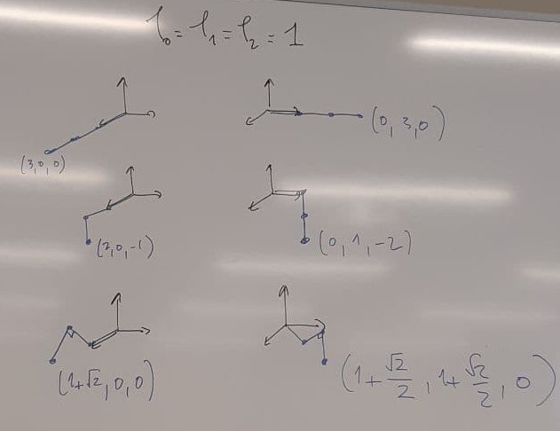
Projet